Au-Cu Alloy

In this example, we will be looking at the classic Au-Cu example from the CLEASE documentation, but run with the GUI instead. We will be using a Face-Centered Cubic (FCC) Au-Cu alloy. In you have not used CLEASE before, we recommend that you start by reading the original example from the CLEASE documentation.

First step is to launch the notebook, see Launching the GUI.

Concentration

The first step is the specify the elements we’re working on. At the time of writing, it is not possible to specify the concentration ranges, but that is coming soon.

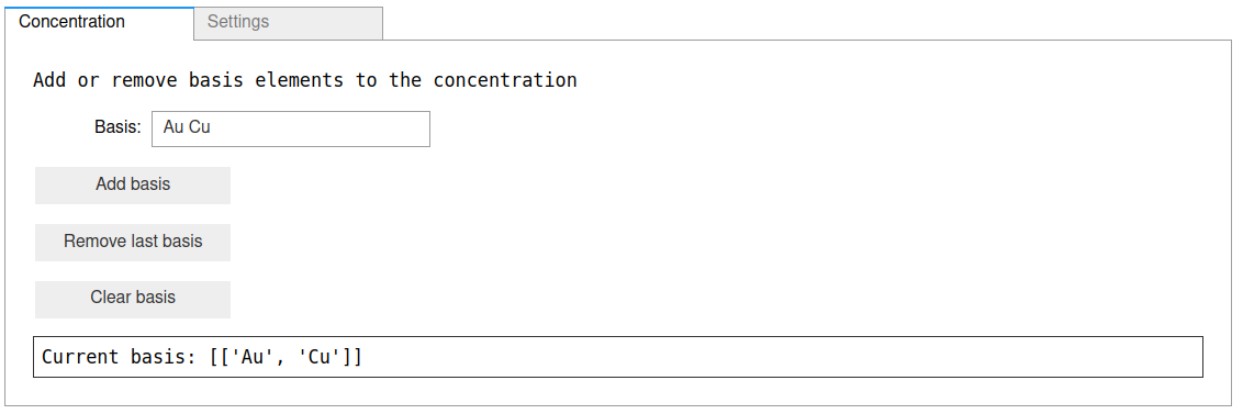
First, specify the basis as Au Cu, and click the Add basis button, and your concentration pane should look something like this:

Settings

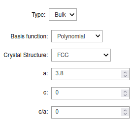
Next, we have to specify the Cluster Expansion (CE) settings. Go to the Settings pane. Set the Crystal Structure to FCC, and set a to 3.8. Leave the rest of the settings to their default values. The crystal settings should look like this:

Then, click on the Make Settings above to construct the CE settings. After the Settings have been made, check the status bar in the bottom, which should have a checkmark at the Settings available? indicator. The status indicator should now look like this:

Finally, let’s save our settings object, so we can use it later. To do that, simply click the Save settings button. If you need to load the settings later, click the Load settings button.

Note

If you ever construct a database, and then later change the settings, (e.g. to adjust the cluster cutoffs), you may need to reconfigure the database. To do this, simply click on the Reconfigure DB button in the settings page.

Creating New Structures

Next, we need to create some structures, so that we cen eventually start fitting our CE model.

Go to the New Structures tab. Here, we can create new structures with different modes. The default mode is to generate random structures at random concrentations. To get started, let’s make 20 new structures, so put 20 in the field No. struct per gen, and click the Generate buton. This will make the 2 end points (pure Au and pure Cu), as well as 18 randomized structures. You can generate more structures by clicking the button again, which will probably become relevant later, if our fit is not satisfactory.

Inspection

We can inspect the structures which are present in our database in the Inspect DB tab. Simply click the Show DB content to see the list of available structures.

An empty querry box means showing all of the structures in the database. For more details on how to construct queries, please see here.

They can be visualized using the Open in ASE GUI tab, which will open an external window. For more information on the ASE GUI, please refer to the ASE GUI documentation.

Calculations

Warning

For educational purposes, a tab for doing EMT calculations has been included. This should not be used to any production purposes. Instead, results need to be populated into the database manually, such as demonstrated on in the CLEASE documentation.

For demonstration purposes, we will use the built-in EMT calculator in this example. Click the Calculate with EMT to run EMT on all the generated structures. And don’t worry about clicking the button multiple times, only structures with no “final” counterpart will be run. Once the calculations are finished, they are automatically placed back into the database.

ECI

The effective cluster interactions (ECI) are the coefficients we attribute to any given cluster, in order to predict energies on new structures. We can fit these to our pre-calculated data in the ECI tab.

Here, we have two fitting algorithm options: LASSO (also known as \(\ell_1\)) ans \(\ell_2\). In this case, we will just use \(\ell_1\) regularization. In the \(\ell_1\) regularization scheme, we have a single hyperparameter to optimize: \(\alpha\).

In the GUI, this is pretty simple: tick the Optimize hyperparameter box, and let’s set the Spacing type to Logarithmic Spacing, min to 1e-8, max to 1, and steps to 100. This optimizes our ECI values with 100 different alpha values in the range [1e-8; 1] with logarithmic spacing, i.e. the sampling density will be lower in the lower ends than in the higher end. Your ECI page should look something along these lines:

Finally, click on the Fit ECI button to start the hyperparameter optimization. Once the optimization is complete, the status bar in the bototm should have a green check mark by the ECI available? indicator. This means, that the ECI values which best fit our data set has been selected, and is ready to be used for Monte-Carlo sampling.

You can see how good of a fit you got in the Fit Plots tab. For example, here is a correlation plot with 40 structures:

The “DFT” energies (in this case EMT) are the true values we attempt to fit, and are situated along the x-axis. The CE energies are along the y-axis. Ideally, these points should be as close to the \(x = y\) line as possible, but that is determined by how good fits we are able to obtain.

Supercells

One of the nice things about cluster expansion, is that it allows us to perform calculations on supercells we would normally not be able to run with regular DFT, especially when combined with techniques such as Monte Carlo sampling.

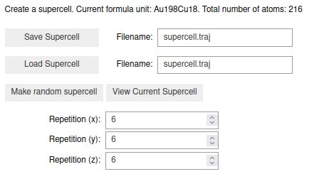
Go to the Supercell tab, and select the size of the cell. The repititions in the \((x, y, z)\) directions are relative to the primitive cell. Let’s make a (6x6x6) supercell. This gives us a new atoms object with 216 atoms. The page should, besides the specific ratio of Au and Cu atoms, looks like this:

We can now use the bottom panel to specify a ratio of Au and Cu atoms. Let’s do the 50/50 cell, i.e. 108 Au and 108 Cu atoms.

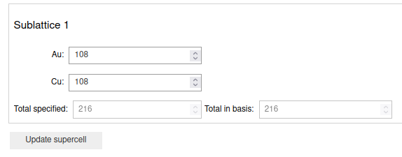
Finally, click the Update Supercell button to set the number of Au and Cu atoms. You should now have a green check mark in the Supercell available? indicator in the status bar.

Monte Carlo

Note

Presently, the GUI only supports regular Monte Carlo sampling.

With settings, ECI and supercell available, we can proceed to performing a Monte-Carlo (MC) sampling of the supercell we just made.

In the Monte Carlo tab, we see a few options. The first is the Step mode, where we have the options sweeps or steps. 1 sweep is defined as running N number of steps, where N is the number of atoms in the supercell. Let’s leave it on sweeps.

Next, we set the number of sweeps, let’s set that to 3. That means, in this case, we’ll run \(3 * 216 = 648\) steps in our Monte Carlo simulation. Finally, let’s increase the number of temperature steps to 100. Once you’re satisfies with your MC settings, click the Run MC button.

We can use the Plotting tab to visualize the run. A good indicator of whether the MC sampling was sufficient, is the Accept Rate, which should be a smoothe downwards curve, which eventually flattens at close to 0.0. In this case, we found an accept rate that looked something like:

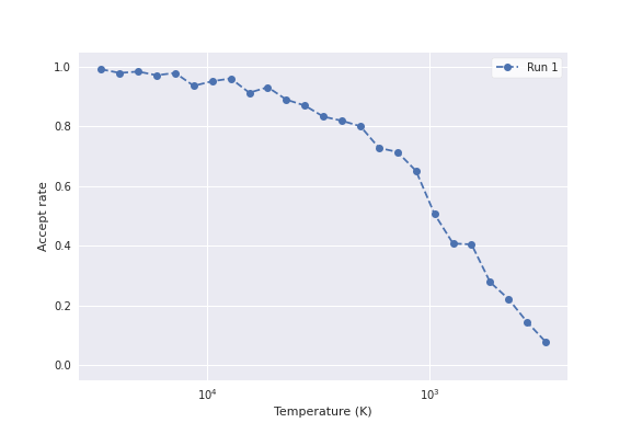
This curve is clearly not very smoothe, which indicates that the number of iterations we ran was insufficient to reach convergence. You can go back and re-run the MC with more steps, to further improve your convergence.

To see the current state of the supercell, go back to the Supercell tab and click on the View current supercell button, which will display the latest configuration which was found in the MC run. You can export the supercell into a file with the Save Supercell button.